\(\renewcommand{\AA}{\text{Å}}\)
fix qbmsst command
Syntax
fix ID group-ID qbmsst dir shockvel keyword value ...
ID, group-ID are documented in fix command
qbmsst = style name of this fix
dir = x or y or z
shockvel = shock velocity (strictly positive, velocity units)
zero or more keyword/value pairs may be appended
keyword = q or mu or p0 or v0 or e0 or tscale or damp or seed or f_max or N_f or eta or beta or T_init
q value = cell mass-like parameter (mass^2/distance^4 units)
mu value = artificial viscosity (mass/distance/time units)
p0 value = initial pressure in the shock equations (pressure units)
v0 value = initial simulation cell volume in the shock equations (distance^3 units)
e0 value = initial total energy (energy units)
tscale value = reduction in initial temperature (unitless fraction between 0.0 and 1.0)
damp value = damping parameter (time units) inverse of friction gamma
seed value = random number seed (positive integer)
f_max value = upper cutoff frequency of the vibration spectrum (1/time units)
N_f value = number of frequency bins (positive integer)
eta value = coupling constant between the shock system and the quantum thermal bath (positive unitless)
beta value = the quantum temperature is updated every beta time steps (positive integer)
T_init value = quantum temperature for the initial state (temperature units)
Examples
# (liquid methane modeled with the REAX force field, real units)
fix 1 all qbmsst z 0.122 q 25 mu 0.9 tscale 0.01 damp 200 seed 35082 f_max 0.3 N_f 100 eta 1 beta 400 T_init 110
# (quartz modeled with the BKS force field, metal units)
fix 2 all qbmsst z 72 q 40 tscale 0.05 damp 1 seed 47508 f_max 120.0 N_f 100 eta 1.0 beta 500 T_init 300
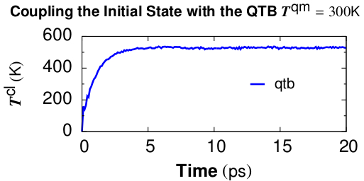
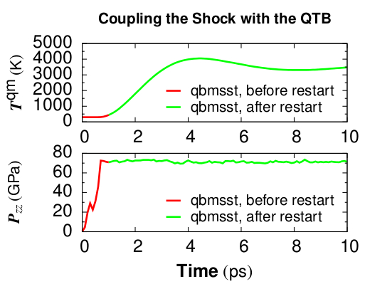
Two example input scripts are given, including shocked \(\alpha\textrm{-quartz}\) and shocked liquid methane. The input script first equilibrates an initial state with the quantum thermal bath at the target temperature and then applies fix qbmsst to simulate shock compression with quantum nuclear correction. The following two figures plot relevant quantities for shocked \(\alpha\textrm{-quartz}\).

Figure 1. Classical temperature \(T_{cl} = \sum \frac{m_iv_i^2}{3Nk_B}\) vs. time for coupling the \(\alpha\textrm{-quartz}\) initial state with the quantum thermal bath at target quantum temperature \(T^{qm} = 300 K\). The NpH ensemble is used for time integration while QTB provides the colored random force. \(T^{cl}\) converges at the timescale of damp which is set to be 1 ps.

Figure 2. Quantum temperature and pressure vs. time for simulating shocked \(\alpha\textrm{-quartz}\) with fix qbmsst. The shock propagates along the z direction. Restart of the fix qbmsst command is demonstrated in the example input script. Thermodynamic quantities stay continuous before and after the restart.
Description
This command performs the Quantum-Bath coupled Multi-Scale Shock Technique (QBMSST) integration. See (Qi) for a detailed description of this method. QBMSST provides description of the thermodynamics and kinetics of shock processes while incorporating quantum nuclear effects. The shockvel setting determines the steady shock velocity that will be simulated along direction dir.
Quantum nuclear effects (fix qtb) can be crucial especially when the temperature of the initial state is below the classical limit or there is a great change in the zero point energies between the initial and final states. Theoretical post processing quantum corrections of shock compressed water and methane have been reported as much as 30% of the temperatures (Goldman). A self-consistent method that couples the shock to a quantum thermal bath described by a colored noise Langevin thermostat has been developed by Qi et al (Qi) and applied to shocked methane. The onset of chemistry is reported to be at a pressure on the shock Hugoniot that is 40% lower than observed with classical molecular dynamics.
It is highly recommended that the system be already in an equilibrium state with a quantum thermal bath at temperature of T_init. The fix command fix qtb at constant temperature T_init could be used before applying this command to introduce self-consistent quantum nuclear effects into the initial state.
The parameters q, mu, e0, p0, v0 and tscale are described in the command fix msst. The values of e0, p0, or v0 will be calculated on the first step if not specified. The parameter of damp, f_max, and N_f are described in the command fix qtb.
The fix qbmsst command couples the shock system to a quantum thermal bath with a rate that is proportional to the change of the total energy of the shock system, \(E^{tot} - E^{tot}_0\). Here \(E^{etot}\) consists of both the system energy and a thermal term, see (Qi), and \(E^{tot}_0 = e0\) is the initial total energy.
The eta (\(\eta\)) parameter is a unitless coupling constant between the shock system and the quantum thermal bath. A small \(\eta\) value cannot adjust the quantum temperature fast enough during the temperature ramping period of shock compression while large \(\eta\) leads to big temperature oscillation. A value of \(\eta\) between 0.3 and 1 is usually appropriate for simulating most systems under shock compression. We observe that different values of \(\eta\) lead to almost the same final thermodynamic state behind the shock, as expected.
The quantum temperature is updated every beta (\(\beta\)) steps with an integration time interval \(\beta\) times longer than the simulation time step. In that case, \(E^{tot}\) is taken as its average over the past \(\beta\) steps. The temperature of the quantum thermal bath \(T^{qm}\) changes dynamically according to the following equation where \(\Delta_t\) is the MD time step and \(\gamma\) is the friction constant which is equal to the inverse of the damp parameter.
The parameter T_init is the initial temperature of the quantum thermal bath and the system before shock loading.
For all pressure styles, the simulation box stays orthorhombic in shape. Parrinello-Rahman boundary conditions (tilted box) are supported by LAMMPS, but are not implemented for QBMSST.
Restart, fix_modify, output, run start/stop, minimize info
Because the state of the random number generator is not written to binary restart files, this fix cannot be restarted “exactly” in an uninterrupted fashion. However, in a statistical sense, a restarted simulation should produce similar behaviors of the system as if it is not interrupted. To achieve such a restart, one should write explicitly the same value for q, mu, damp, f_max, N_f, eta, and beta and set tscale = 0 if the system is compressed during the first run.
The cumulative energy change in the system imposed by this fix is included in the thermodynamic output keywords ecouple and econserve. See the thermo_style doc page for details.
This fix computes a global scalar which can be accessed by various output commands. The scalar is the same cumulative energy change due to this fix described in the previous paragraph. The scalar value calculated by this fix is “extensive”.
The progress of the QBMSST can be monitored by printing the global scalar and global vector quantities computed by the fix.
As mentioned above, the scalar is the cumulative energy change due to the fix. By monitoring the thermodynamic econserve output, this can be used to test if the MD timestep is sufficiently small for accurate integration of the dynamic equations.
The global vector contains five values in the following order. The vector values output by this fix are “intensive”.
[dhugoniot, drayleigh, lagrangian_speed, lagrangian_position, quantum_temperature]
dhugoniot is the departure from the Hugoniot (temperature units).
drayleigh is the departure from the Rayleigh line (pressure units).
lagrangian_speed is the laboratory-frame Lagrangian speed (particle velocity) of the computational cell (velocity units).
lagrangian_position is the computational cell position in the reference frame moving at the shock speed. This is the distance of the computational cell behind the shock front.
quantum_temperature is the temperature of the quantum thermal bath \(T^{qm}\).
To print these quantities to the log file with descriptive column headers, the following LAMMPS commands are suggested.
fix             fix_id all msst z
variable        dhug    equal f_fix_id[1]
variable        dray    equal f_fix_id[2]
variable        lgr_vel equal f_fix_id[3]
variable        lgr_pos equal f_fix_id[4]
variable        T_qm    equal f_fix_id[5]
thermo_style    custom  step temp ke pe lz pzz econserve v_dhug v_dray v_lgr_vel v_lgr_pos v_T_qm f_fix_id
It is worth noting that the temp keyword for the thermo_style command prints the instantaneous classical temperature \(T^{cl}\) as described by the fix qtb command.
Restrictions
This fix style is part of the QTB package. It is only enabled if LAMMPS was built with that package. See the Build package page for more info.
All cell dimensions must be periodic. This fix can not be used with a triclinic cell. The QBMSST fix has been tested only for the group-ID all.
Default
The keyword defaults are q = 10, mu = 0, tscale = 0.01, damp = 1, seed = 880302, f_max = 200.0, N_f = 100, eta = 1.0, beta = 100, and T_init=300.0. e0, p0, and v0 are calculated on the first step.
(Goldman) Goldman, Reed and Fried, J. Chem. Phys. 131, 204103 (2009)
(Qi) Qi and Reed, J. Phys. Chem. A 116, 10451 (2012).